What's going on everybody! Welcome again to my blog! This is the second post in the Machine Learning Series of Articles. I hope you liked the previous articles in this category. The previous post was a brief introduction to Machine Learning. If you have not yet read the previous post, you may refer it here. If you like the posts, please do give feedback using the feedback form provided at the end of the articles. Also please share the articles over your preferred social media using the share buttons provided below the articles. Also please do suggest any improvements or additions I may make to get the articles even better. So, without any further delay, let us get to the topic of this article, Linear Regression.

Before getting into the algorithm of Linear Regression, let us first understand what exactly the term means. The term Linear Regression is created by mixing of two different words: Linear and Regression. So, intuitively, we can guess that the word Linear suggests that it is somewhat related with Linearity, that is related to straight lines. I shall come to this later in the article. But first, it is imperative to know about Regression.

According to an article by Towards Data Science, Regression is defined as: Regression is a method of modelling a target value based on independent predictors. This may sound a bit confusing. Let me explain it in a very simple manner. I shall give an example of a real-world problem to make this definition clear. Suppose, you are planning to buy a new house. So, what shall be your first step? You will be contacting a broker or a middleman who will be having information about the available houses for sale. He showed you some houses. You loved some of the houses and asked the middleman about an estimated price of each of the houses. So, the middleman will give you an estimated cost per house. How does he determine the estimation? Yes, you got it right! He will be guessing the prices of each house based on some properties of the particular house like the size of the house, what locality the house is at, how many rooms are available in the house, how advanced and attractive the design of the house is, and so on. These properties are also called Features. So, based on the features the house has, he will be giving you an estimate of the cost. This is exactly what the definition states. Read the definition again, which states, Regression is a method of modelling a target value (the price of the house in our example) based on independent predictors (the features of the house in our example. The features are independent, for instance, size of the house and locality of house are not inter-dependent). Thus, this method is mostly used for forecasting and finding out cause and effect relationship between variables. The method of Regression is used when the prediction is continuous and not discrete.

So, knowing what Regression means, let us talk about Linear Regression. Linear Regression, commonly called Simple Linear Regression is a type of Regression analysis in which the number of independent predictors is one. That is, for predicting the target value, we use only a single feature, for instance, predicting our house price using only the size of the house or only the locality of the house. There is another variant of Regression, called Multivariate Regression, which deals with predicting the target variable using multiple features (as in our example of housing pricing). We shall talk about this variant in later posts. Talking about Simple Linear Regression, the predictor variable, that is the features are conventionally denoted by (X), and the target variables are denoted by (Y). And it is intuitive that as we are trying to find the value of (Y) from (X), they must be related, which makes (Y) as the Dependent variable and (X) as the independent variable.

Now, let me ask you a quick question:
Suppose we are given with the values of X as [1, 2, 3, 4, 5] and the corresponding values of Y as [3, 5, 7, 9, 11]. And if I ask you to guess the value of Y when X = 8, what shall be your answer?
So, this was not a difficult task for you. You will instantly answer that the value of Y will be 17. But the main question is, how did you come to this conclusion? And the answer is simple, the values X and Y are related by the formula:

Y = 2*X + 1

Thus for the value of X as 8, we get the value of Y as 17.
Now, as you must have already guessed, the relationship between X and Y in Simple Linear Regression is Linear, thus the name Linear Regression. Thus the relationship between X and Y can be generally denoted as:

Y = a₀ + a₁X ....... (1)

This equation is similar to the equation of a straight line (Y = mX + c). Here, a₀ and a₁ are known as the co-efficients of Linear Regression. Now, let me modify the above equation numbered (1), and write X as X₁ and introduce a term X₀ which will be always equal to one. Thus the equation can be modified to:

Y = a₀X₀ + a₁X₁ ......... (2)

Y = a_iX_i ..........(3)

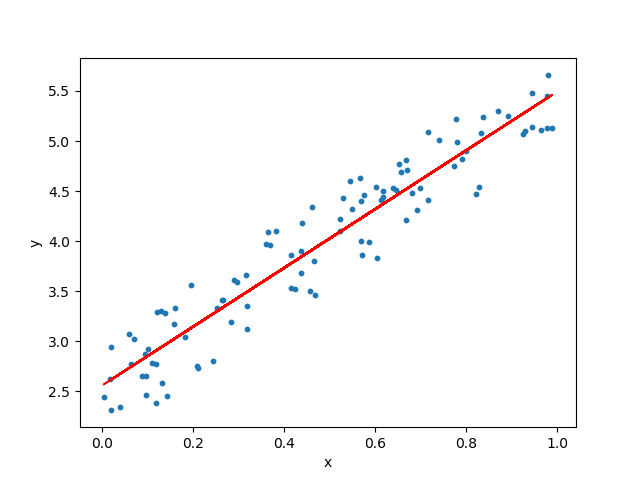
The aim of our algorithm is to find the best values of a₀ and a₁. Thus, as in the picture provided at the start of the article, we will be provided with all the X values (denoted by blue dots in the picture). Based on the corresponding Y values, we will be finding out the values of the co-efficient such that it will generate the given line (in red) which best fits all the data points in the graph. And then, given a new input X, we will substitute the value of X in the equation of the obtained line to predict the value of Y. Here, it is important to note that the line generated does not always fit all the data points. It is an approximation of the relation between X and Y. Thus it is also called the Best Fit Line. Now, as discussed the approaches in the previous post, could you guess the type of approach (Supervised, Unsupervised or Reinforcement) of this method?
Yes! You guessed it right! It is a Supervised approach. How? Because we are provided with samples X and Y from which the device will learn and predict from other unseen values of X (remember that I had provided you with a list of different X and corresponding Y after which you guessed the value of Y for a completely unseen example of X).

Before going into the algorithm, it is necessary to understand a couple of terms which will be useful throughout our study of Machine Learning:

1) Cost Function:
This is a very important concept used in Machine Learning to facilitate the learning process. During the Learning phase of the device, the device will start with random initialization of the coefficients and find the output. Now, it will try to check the output calculated with the actual output. The Cost of a particular output can be explained as how much error is there in the output of the device, that is how much far is the output of the device than the actual output. Thus, it will help measure the degree of correctness, or how much accurate the prediction of the model is.
There are many ways, or rather functions which are used in Machine Learning to compute the cost of the output. Some of them being Mean Squared Error, Binary Cross-Entropy, Exponential Cost, Relative Entropy, Sparse Categorical Cross-Entropy and a lot more. These cost functions are selected based on the algorithm we are using. For our purpose, for now, the most commonly used cost function for Linear Regression is the Mean Squared Error function. This function is defined as:

C(Prediction_i , Y_i) = (Y_i - Prediction_i)²

And, the total cost will be defined as:

C(Prediction , Y) = (Y_i - Prediction_i)²
where n is the number of training examples we provide to the algorithm, Prediction is the output predicted by the device and Y is the actual output of the i^th training example

As you must have already understood it, the aim of the algorithm now scales to finding the value of a₀ and a₁ such that the value of the cost of the algorithm is minimum.

Now, the question arises, How to minimise the cost and find the optimal co-efficients?
For that, let us look at another important concept in Machine Learning:

2) Gradient Descent: Gradient Descent is a method of updating the values of a₀ and a₁ to minimise the value of the Cost Function. Now, according to your mathematical knowledge, could you guess the shape of the curve of the Cost Function (Mean Squared Error) which we used above?
You are absolutely correct! The shape of the curve will be convex, because it is a Quadratic Function. So, to find the minimum value of the quadratic function, which is the method widely used? We will be differentiating the function partially with respect to a₀ and a₁, and updating the values of a₀ and a₁ as shown in the following equations:

Here, J is the Cost Function, pred_i is the device prediction of the i^th example and n is the number of examples

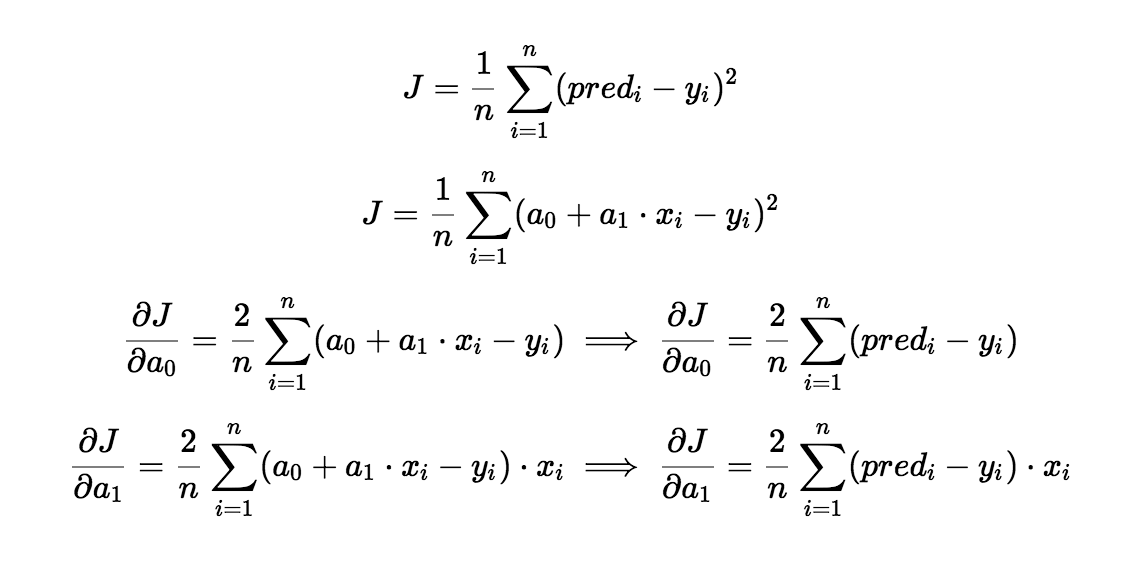
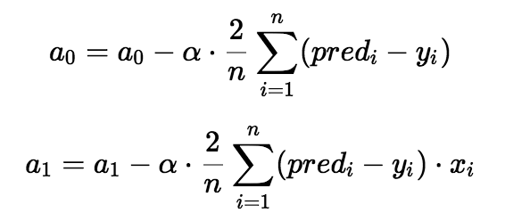
So, you got the equations of the Gradient Descent. But, there is a symbol in the equations. This is known as the Learning Rate. Intuitively, it shows how big your step must be to come to the minimum value of the cost function. You will understand this further in the post as you read on. The value of the Learning Rate is a Hyper-Parameter and is chosen by us during the training. Generally, a value of about 0.01 is taken, but the value of alpha completely depends upon the problem and may change. Now, let us understand how the Gradient Descent works:

Let us take a particular example of a curve of the cost function:

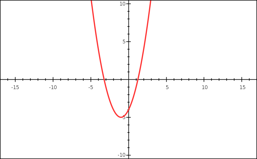
Now, as discussed earlier, let the computer start with a random value of a₀ and a₁. Let us pick a random point on the curve, say (3,5). For a₀ = 3, we get cost = 5. Also, the gradient at (3,5) is positive (intuitive from the graph). So, using the equation provided above, for a positive alpha, the new value of a₀ will be to the left of the present value. The value of alpha tells the algorithm how much to the left must it go, which is also known as the step size. Thus, it is a good practice to test the algorithm with different values of alpha to find which value suits it the most. Moreover, choosing a good value of alpha is imperative as taking big steps will make the algorithm oscillate but never reach the minimum and taking too small alpha may make the algorithm slower. It can be intuitively understood from the images:

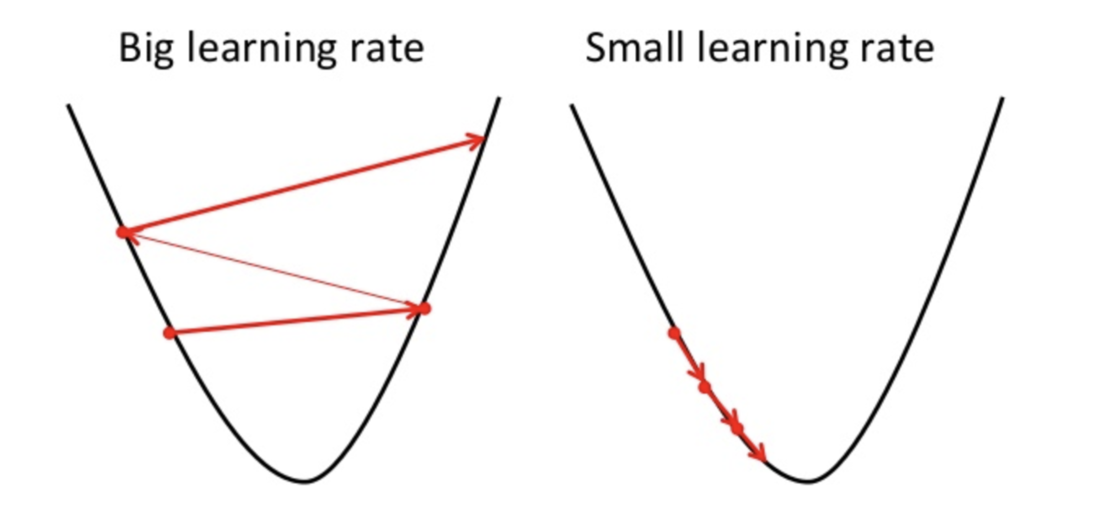
Thus, we can run the above updations simultaneously for a₀ and a₁ for either a specified number of iterations or until the value of the cost function becomes minimum. The line obtained from these coefficients is the required Best Fit Line. This was a thorough theoretical introduction of Simple Linear Regression Algorithm. We shall talk about the implementation of this algorithm in subsequent articles.

Please let me know your feedback regarding this article and if you liked the article, please share it on your preferred social media using the links provided below. Also, do suggest me about any improvements which I may implement to make the blog even better using the feedback form provided. Further, I will be writing about other Machine Learning algorithms in future posts as well as an implementation of Linear Regression (both self-implemented as well as using Scikit-Learn). Please stay tuned! Until then, have a great time!