What's going on everybody! Welcome again to my blog! In the previous articles, I had talked in detail about Tokenizers and Positional Embeddings. In this article, we shall look a bit into Computer Vision and an interesting implementation of One Shot Face Recognition. In case you feel any difficulty during the implementation provided in this article, feel free to let me know through the contact form provided below the article. If you like this article, please make sure to give it some applauses and also share it over your preferred social media using the links provided. Do provide your feedback or suggestions which may help me improve the blog even better. So, cutting off the talks, let us jump straight to the implementation.

But now, what is One Shot Face Recognition? Normally, when we train any Machine Learning algorithm, we require lots of similar type of data for the algorithm to train. But, this approach is not effective for tasks like face recognition. Face Recognition aims not only to detect a human face in a given image, but also to recognize whose face it is in the image. But to train such an algorithm in the traditional approach, we will require tens, if not hundreds of images of each person as a different class and train the algorithm to learn to classify the faces. This is not practical as one might not be able to get so many images of a single person. Also, what if we want to add more person classes in it? We will have to get pictures of the new person and train the model as a whole all over again. Same will be the case if we want to remove a person as a class. To overcome such drawbacks, we imply One Shot Approach for image recognition. This approach enables us to recognize faces using a single image for each person. This image will be used as a reference image and the actual image will be compared with the reference images and will be classified based on the most matching reference image.

Approach

The following approach will be used for implementing out model:

1) Creating a feature extraction model:

The Feature Extraction model will take an image as an input and convert it into an encoded vector. These encodings will represent the features extracted from the image. We may use any model of our choice which is able to convert images to vectors. Normally, CNN based deep models are used. In this implementation, we will used a pre-trained InceptionV3 model from the Keras Application API and fine-tune the model to out specific task. You may also choose a different model, or choose to train the model from scratch instead of using a pre-trained one.

2) Implementing a Siamese Network with the Feature Extraction model as the Base Model:

Now what is a Siamese Network? A Siamese Network is used when we want to compare two different inputs to a model, instead of just feeding one input and getting the output. Let me explain it to you using an image

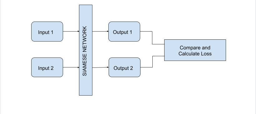
So, as seen in the above image, Siamese Network takes more than one input, and gives out same number of outputs. These outputs are then compared and necessary functions are then performed on these outputs. The SIAMESE NETWORK block in this image is nothing but a number of Feature Extraction model architectures, ideally same number as the number of inputs. Each input is passed through their dedicated model and features are extracted. The weights and parameters of all these models are shared, that is, there is a single set of parameters which all these models use. Here, instead of having different models, we will have only one model architecture with one set of weights and we will pass all the input images turn by turn and save the features. It is essentially the same thing!

3) Preparing a Loss Function:

To compare the outputs, we will require a loss function which will essentially calculate the similarity between the outputs. Less the loss value, more the similarity. So what shall the loss function be? What we can do, is that we can give one reference image and our actual image to the Siamese Network and then design a loss which will calculate the absolute distance between the two set of features obtained. We will have to then decrease this absolute distance loss to increase the accuracy of the model. Lesser the distance, more the similarity. This is a good approach, but we will not use this. Instead, we will try to teach the model something more! Instead of just teaching our model to recognize similar faces, we will also teach the model to differentiate non-similar faces. How can that be done? Let us say, we take three images as input. One will be our actual image which we need to recognize. Let us call this as the Anchor Image (this is the actual term for such images). Other image will be of the same person as in the Anchor Image. This image is called as the Positive Image. And the third image will be of a completely different person. This image is termed as the Negative Image. We will feed these images to our Siamese Network and get three different set of Features. Now, while training, we will try to increase the distance between the anchor and the negative image and decrease the distance between the positive and the anchor image features, simultaneously. Yes! This should work! The loss which I am talking about here, is called the Triplet Loss. Mathematically, the Triplet Loss is defined as

Here, the function is nothing but the feature extractor function, which will be the InceptionV3 model we will be using in our implementation. are the Anchor, Positive and Negative Image inputs. Moreover, is a hyperparameter. We calculate the maximum of the loss with just to keep the loss positive and not take any action in case the loss becomes negative. Here, decreasing this loss will be the aim of the training, as decreasing this loss will increase the distance between anchor and negative images, and decrease distance between anchor and positive images.

Let's get to the implementation now!

So, let us start the implementation now! We will be using Keras and Numpy libraries for the implementation. We will not require any additional libraries for this. You can install the Tensorflow and Numpy using the following command:

~$ pip install tensorflow numpy

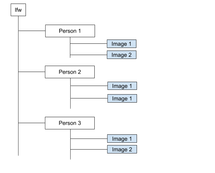
We will now collect data to train our model on. We will be using the LFW Face Database for this. This database contain about 13,000 faces of different people. The download size of this dataset is about 180M zipped (.tgz file). You can download the dataset using the following

~$ wget http://vis-www.cs.umass.edu/lfw/lfw.tgz    # Assuming Linux Systems
~$ tar -xf lfw.tgz                                 # Untar the file
~$ rm lfw.tgz                                      # Remove the original file to save disk space

The above commands will untar the file and a folder named will be created. This folder has the following structure

So, we got the data. Our next step will be to prepare our dataset for preprocessing. For this, we will require one anchor image, one positive image, and one negative image. We will do this by walking through all the folders, selecting each image as anchor, selecting other image from the same folder as a positive and one image from any other random folder as the negative image. But first, let us import all the required libraries

import tensorflow as tf
from tensorflow.keras import backend as K
from tf.keras.applications.inception_v3 import preprocess_input
from tf.keras.applications import InceptionV3
import numpy as np
import os
from tqdm import tqdm
import random
import matplotlib.pyplot as plt   # Optional

Now, let us create a utility function to generate the (Anchor, Positive, Negative) image pairs

def make_pn_pairs(pairs=pn_pairs, dir='lfw'):
  pn_images = []
  for pair in pairs:
    l = os.listdir(dir+'/'+pair[0]+'/')
    for i in l:
      image = dir+'/'+pair[0]+'/'+i
      positive = dir+'/'+pair[0]+'/'+random.choice(l)
      n = os.listdir(dir+'/'+pair[1]+'/')
      negative = dir+'/'+pair[1]+'/'+random.choice(n)
      pn_images.append((image, positive, negative))

  return pn_images

pn_images = make_pn_pairs()
print(pn_images[0])
assert all(((x[0].split('/')[1] == x[1].split('/')[1]) and (x[1] != x[2])) for x in pn_images)

The above function will create a list of tuples, where each tuple is the path to (Anchor, Positive, Negative) images. We can use these paths to load the images later. As the next step, as we are using the InceptionV3 model, we will have to preprocess our input images in the same manner as described in the InceptionV3 paper. We could self implement it, but Keras already provides an API for preprocessing an image for using it with the InceptionV3 model. We shall create a utility function to preprocess an input pair

def preprocess_image_pair(image_pair):
  img1, img2, img3 = tf.io.read_file(image_pair[0]), tf.io.read_file(image_pair[1]), tf.io.read_file(image_pair[2])
  img1, img2, img3 = tf.image.decode_jpeg(img1, channels=3), tf.image.decode_jpeg(img2, channels=3), tf.image.decode_jpeg(img3, channels=3)
  img1, img2, img3 = tf.image.resize(img1, (299, 299)), tf.image.resize(img2, (299, 299)), tf.image.resize(img3, (299, 299))
  img1, img2, img3 = preprocess_input(img1), preprocess_input(img2), preprocess_input(img3)
  return np.array(img1, ndmin=4), np.array(img2, ndmin=4), np.array(img3, ndmin=4)

data = preprocess_image_pair(pn_images[46])
print(data[0].shape)
print(data[1].shape)
print(data[2].shape)

Here, we will require the image size to be as accepted by the Inception Model. Hence, we resize it to this size. After that, we do the preprocessing on the images based on the standard preprocessing done while training the InceptionV3 model. The function essentially does the following

def preprocess_input(x):
    x /= 255.           # Elementwise division with 255.0
    x -= 0.5            # Elementwise subtraction with 0.5
    x *= 2.             # Elementwise squaring
    return x
# No need to implement this function. This is just for reference

We will now create our Feature Extraction Model which will be used as the Base Model for our Siamese Network. Here, we will use the InceptionV3 model along with the classification head. This will output a dimensional vector as the features of each image

image_model = tf.keras.applications.InceptionV3(include_top=True, weights='imagenet')   # weights=None for random initialization
new_input = image_model.input
hidden_layer = image_model.layers[-1].output

image_features_extract_model = tf.keras.Model(new_input, hidden_layer)
print(image_features_extract_model.layers)

If you have used , it will download pre-trained InceptionV3 model on your system. The download size is about 95-100M. Next, we will have to create custom Keras Layers for our Siamese Network model. We will also implement the Triplet Loss as a Layer insted of a Function. For this, we will run the following code

class SiameseNet(tf.keras.layers.Layer):

  def __init__(self, model):
    super().__init__()
    self.model = model

  def call(self, img):
    feats = self.model(img[0])
    nfeats = self.model(img[2])
    pfeats = self.model(img[1])
    final = tf.stack([feats, pfeats, nfeats])
    return tf.transpose(final, perm=[1,2,0])


class TripletLoss(tf.keras.layers.Layer):

  def __init__(self, alpha):
    self.alpha = alpha
    super().__init__()

  def call(self, features):
    pos = K.sum(K.square(features[:,:,0] - features[:,:,1]))
    neg = K.sum(K.square(features[:,:,0] - features[:,:,2]))
    base_loss = pos - neg + self.alpha
    return K.maximum(base_loss, 0.0)

Here, the Layer will take a list of images as input, pass all these images through the Base Model and return a stack of features corresponding to each images. The Layer will take the features as input and using the formula given earlier in the article, it will calculate the distance between each features to return the final loss.

Now, let us create our actual model! We will use the Keras Model API for this, just like we did in the InceptionV3 Model.

image_input = tf.keras.layers.Input(shape=(299,299,3), name='image_input')
negative_input = tf.keras.layers.Input(shape=(299,299,3), name='negative_input')
positive_input = tf.keras.layers.Input(shape=(299,299,3), name='positive_input')

siamese = SiameseNet(image_features_extract_model)([image_input, positive_input, negative_input])
loss = TripletLoss(alpha=1)(siamese)
model = tf.keras.Model(inputs=[image_input, positive_input, negative_input], outputs=loss)

Now, let us compile our model. Here, to provide it a loss, we will implement an identity loss, which will just return the mean of the predicted value, just to make sure that it does not contribute to the training.

def identity_loss(y_true, y_pred):
  return K.mean(y_pred)


model.compile(optimizer = tf.keras.optimizers.Adam(lr=1e-5), loss = identity_loss)
print(model.summary())

As the final preparation before starting the training, we will prepare the data in the required input format. We will create three Numpy Arrays corresponding to each Anchor, Positive and Negative Images. Due to compute restrictions, I have only been able to use 500 images out of the 13000+ images. But you can use all if you have the proper resources. We shall run the following block of code for this

images, positives, negatives = [], [], []

for pair in tqdm(pn_images):
  data = preprocess_image_pair(pair)
  images.append(data[0])
  negatives.append(data[2])
  positives.append(data[1])

images = np.concatenate(images)
positives = np.concatenate(positives)
negatives = np.concatenate(negatives)

The shape of and vectors will be each. We convert this to numpy array because the training will require it in this format. If you want, you can also assign a small set of images from this as the validation set.

Now, we are pretty much done with all the preparations. We can start the training process now. But before that, let us set one more option for our training. We will configure a Scheduler for our training process. In case you do not know what a Scheduler is, a Scheduler is a utility which help us make our Learning Rate dynamic. In other words, to facilitate our process of learning, we can change the value of the Learning Rate during a running training process. This is required because sometimes, when the model is sensitive to loss, or maybe when it is close to converging, it may take a longer step than required if the Learning Rate is fixed. But we can decrease the Learning Rate value as the training progresses to ensure proper convergence at the end. This is not always required, but we will use it here. We can create a Learning Rate Scheduler using the Keras Callbacks API.

def scheduler(epoch, lr):     # Reduces LR by a factor of 10 on each epoch
  if epoch == 1:
    return lr
  return lr / 10

callbacks = [
  tf.keras.callbacks.LearningRateScheduler(scheduler, verbose=0)
]

And now we are finally done! Now, we can train the model on our data.

history = model.fit([images, positives, negatives], np.ones(images.shape[0]), batch_size=10, verbose=2, epochs=6, callbacks=callbacks)

Here, you can customize the parameters of batch size and epochs according to the amount of data you are using. Just a final question. Why did we use in place of the ? This is because we do not actually require a in this model as all our calculations are based on the inputs itself. Hence, as it is a required parameter, we will use this pseudo-parameter in place.

As a final step, let us plot the loss values with respect to the number of epochs.

plt.plot(history.history['loss'])
plt.title('Loss')
plt.xlabel('Number of Epochs')
plt.ylabel('Loss')

We will also plot the Learning Rate to check whether it really decreases per epoch

plt.plot(history.history['lr'])
plt.title('Learning Rate')
plt.xlabel('Number of Epochs')
plt.ylabel('Learning Rate')

To use this trained model for prediction, you just need to save the using the following

image_features_extract_model.save('face_recognition_base_model.h5')   # Save

from tensorflow.keras.models import load_model
loaded_model = load_model('face_recognition_base_model.h5', compile=False)      # Load

You can create a wrapper around this model and define a loss for your prediction similar to what we did here. The full implementation as a Jupyter Notebook can be downloaded from here, or you can view the notebook at the Github Repo

Conclusion

So, this was the implementation of One Shot Face Recognition using Keras. You may try experimenting with the hyperparameters to improve the result. Let me know how it goes! Do share your feedback on this article using the form provided below. Also, some applauses would be great if you liked this article. You can share this article on your preferred social media using the share buttons. Do suscribe to receive the latest updates on the blog. I shall write an implementation of a different project next time. Till then, have a great time!